Contents
setMTEXpref('generatingHelpMode',true); % Avoid some artefact (fix issue #5)
mtexdata small
ebsd = ebsd('indexed');
grains = calcGrains(ebsd);
G=gmshGeo(grains);
ebsd = EBSD

 Phase  Orientations     Mineral         Color  Symmetry  Crystal reference frame
     0    1197 (32%)  notIndexed
     1    1952 (52%)  Forsterite  LightSkyBlue       mmm
     2    290 (7.8%)   Enstatite  DarkSeaGreen       mmm
     3    282 (7.6%)    Diopside     Goldenrod     12/m1        X||a*, Y||b, Z||c

 Properties: bands, bc, bs, error, mad, x, y
 Scan unit : um
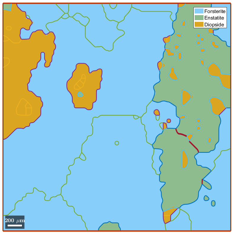
Plot the whole geometry
The whole geometry can be plotted with the usual plot command:
plot(G)
The orientation used for plotting is inherited from the MTEX preferences. It ensures consistency between the two kinds of plot. For instance, if you want to superimpose the grains boundaries defined in G and the original grains:
plot(grains,'noBoundary')
hold on
plot(G)
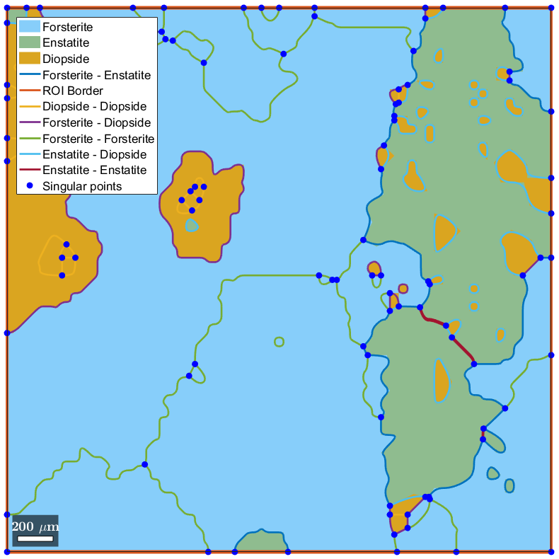
Display singular points
In MTEX2Gmsh, singular points refer to triple points, quadruple point (or even higher order), corners of the RoI and double point at the border of the RoI. Such point can be plotted undividually:
plotSingularPoints(G)
legend('Location', 'NorthWest')
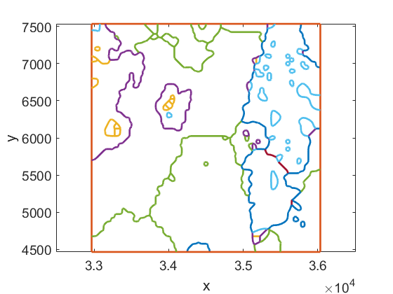
Plot specific grains
Linear indexing helps plotting specific grains. For example, the following plots grains 65 and 67:
figure
plot(G([65 67]))
legend('Location', 'Best')

Alternatively, one can specify the phase to be plotted. E.g:
plot(G('Diopside'))
legend('Location', 'Best')
