Contents

setMTEXpref('generatingHelpMode',true); % Avoid some artefact (fix issue #5)

mtexdata small
[grains, ebsd('indexed').grainId]=calcGrains(ebsd('indexed'));
ebsd(grains(grains.grainSize<3))=[];	% Remove small grains
grains=calcGrains(ebsd('indexed'));
G=gmshGeo(grains);

 
ebsd = EBSD  
 
 Phase  Orientations     Mineral         Color  Symmetry  Crystal reference frame
     0    1197 (32%)  notIndexed                                                 
     1    1952 (52%)  Forsterite  LightSkyBlue       mmm                         
     2    290 (7.8%)   Enstatite  DarkSeaGreen       mmm                         
     3    282 (7.6%)    Diopside     Goldenrod     12/m1        X||a*, Y||b, Z||c
 
 Properties: bands, bc, bs, error, mad, x, y
 Scan unit : um
 

Basic use

The geometry described by the object G can be meshed using the Gmsh software as follows:

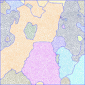
mesh(G,'default.msh')

Open mesh file

The above command results in a 1 element thick mesh, consisting in linear wedge elements (6-node 3D elements. The element size is (roughly) equal to the EBSD resolution.

Constant element size

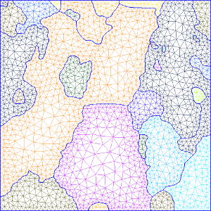
The default element size can be set as follows:

mesh(G,'constant_elmtSize.msh','ElementSize',50)

The resulting mesh cannot be (easily) displayed in MATLAB. Thus, the following illustrates the geometry when opening the mesh file with Gmsh:

Open mesh file

The unit here is the same as the EBSD map (ususally µm).

Size gradient

Let be the local element size at coordinates . The element size can be set as an increasing distance from the grains boundary such that:

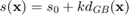
with:

If one wants to mesh with element size equal to 50 at grain boundaries and a slope of k=0.5:

mesh(G,'sizeGradient.msh','ElementSize',50,'gradient',0.5);

Open mesh file

If you need finer control over the element size (for instance if you want to refine the mesh in specific grains), see advanced options for meshing.

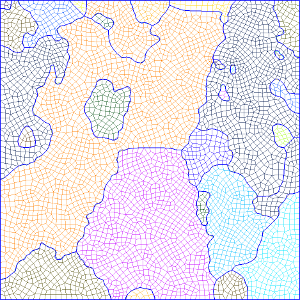
Element size Depending on the curvature of grain boundaries

The local curvature of grain boundaries can be used to set the element size. For instance, the following command use 5 nodes to describe a full circle:

mesh(G,'curvature.msh','Curvature',5);

Open mesh file

Element type

The default element type for meshing is linear wedge. It can be changed to hexahedron (or brick element).

mesh(G,'brick.msh','ElementType','Hex');

Open mesh file

Note: In this case, the mesh will be hex-dominated. Indeed, the resulting mesh may still contain some wedge elements. To avoid it, use 'HexOnly' option instead.

Tetrahedron can also be used:

mesh(G,'tet.msh','ElementType','Tet');

Open mesh file

If you wants to work in 2D only, use triangular ('Tri') or quandrangular ('Quad') elements instead:

mesh(G,'Tri.msh','ElementType','Tri');

Open mesh file

mesh(G,'Quad.msh','ElementType','Quad');

Open mesh file

Again, 'Quad' results in quad-dominated mesh. For pure Quad mesh (no triangle), use 'QuadOnly'.

Element order

The default element order is 1 (linear elements). It can be changed with the ElementOrder option. E.g.:

mesh(G,'brick-quadratic.msh','ElementType','Hex','ElementOrder',2);

Open mesh file

Periodic mesh

Periodic conditions can be used on X or/and Y direction for meshing. It consists in ensuring that nodes at opposite borders are at the same coordinates. This is usually requested for periodic conditions in FEM in order to take into account the medium surrounding the RoI.

mesh(G,'Periodic-x.msh','elementSize',100,'periodic','x');

Open mesh file

mesh(G,'Periodic-xy.msh','elementSize',100,'periodic','both');

Open mesh file

Dump the geometry in an ASCII file

The geometry can be exported into a Gmsh-readable (and somehow human-readable) format using the following command:

savegeo(G,'geometry.geo')

Open geo file

Go back to documentation index

Published with MATLAB® R2013b